Redshift Cost Optimization for SaaS Analytics

The message usually comes from whoever owns the AWS bill, and it is never dramatic. “Redshift is up again this month. Did we onboard someone big?” Nobody onboarded anyone. Nobody shipped a new dashboard. Query volume looks flat on the Grafana board. The bill moved anyway.

That gap between what you think you are paying for and what you are actually paying for is what makes Redshift cost optimization awkward in a SaaS analytics product. You are not running one nightly batch against a warehouse that sleeps the rest of the day. You are serving hundreds of small, latency-sensitive queries that fire whenever a customer opens a dashboard, plus ingestion, plus whatever your BI layer and your connection pool are doing when nobody is watching.

This post covers the levers that genuinely move that number: how the meter works, why idle-looking connections still bill, how to work out which tenant is expensive, and which isolation choices cost more than they save. Where the popular advice is wrong for SaaS specifically, I will say so.

How Amazon Redshift actually charges you

Three buckets, and they behave very differently.

Compute. On Redshift Serverless this is RPU-hours, metered per second. On provisioned clusters it is node-hours, plus separate line items for concurrency scaling and Spectrum.
Storage. Redshift Managed Storage, billed by GB per month, independent of compute. Snapshots are storage too.
Everything else. Cross-region data sharing and snapshot replication, machine learning, data transfer outside the usual in-region S3 paths.

In a SaaS analytics workload compute dominates, often overwhelmingly. And the important part: compute is a function of how long the warehouse is awake and at what capacity, not how many rows you touched. Two teams can scan identical data volumes and get bills that differ by a factor of five, purely because of how their queries arrive.

The billing mechanic that catches SaaS teams out

Read the serverless billing notes properly once and a lot of mysterious spend stops being mysterious. The parts that matter:

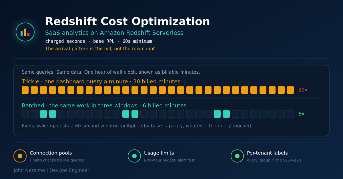
The minimum charge is 60 seconds of resource usage, metered per second beyond that. This is a minimum for the warehouse, not for each individual query.
Usage is recorded when a transaction completes, rolls back, or is stopped. A transaction that runs for hours shows up in your usage view only at the end.
Cancel a query before it finishes and you still pay for the time it ran.
Querying system tables is billed like any other query. Your monitoring loop is a workload.
After a burst, capacity can stay elevated for a period after the load drops. Scale-down is not instant.

Put those together and you reach a conclusion that irritates most engineers: on serverless, ten small queries crammed into one minute are cheaper than the same ten queries spread across ten minutes. Every wake-up costs you a minimum billing window multiplied by your base capacity. That is the opposite of the instinct you have from tuning an OLTP service, where you smooth load out to protect tail latency.

Before you change anything, get the real numbers out of the warehouse rather than out of Cost Explorer, which lags and aggregates.

-- Daily billed RPU-seconds converted to RPU-hours.
-- Multiply by your region's on-demand RPU-hour rate for dollars.
SELECT trunc(start_time) AS day,
       sum(charged_seconds) / 3600::double precision AS rpu_hours
FROM   sys_serverless_usage
GROUP  BY 1
ORDER  BY 1 DESC;

charged_seconds is the column to build cost reporting on. compute_seconds is informative but it is not what the invoice is derived from, and the two can disagree within a given interval. Two constraints worth knowing before you wire this into a dashboard: the view holds roughly a week of history, and it is visible only to superusers. If you want month-over-month trends, UNLOAD it to S3 on a schedule and query the archive with Amazon Athena instead.

Lever one: connections that look idle and are not

This is the one that bites hardest and shows up last, because there is nothing to see. AWS documents it plainly: Redshift Serverless treats all incoming queries as billable user activity, including lightweight health-check queries sent by connection pools. It does not matter whether the statement came from your application, a JDBC driver, or a pooling framework doing its job.

So a pool that fires SELECT 1 every thirty seconds to validate connections is a warehouse that never gets to sleep. Your product has no users at 3am and you are still paying the minimum window, over and over, multiplied by base capacity. HikariCP, Apache Commons DBCP and PgBouncer all have some form of this behaviour, and the defaults are tuned for OLTP databases where a validation query costs nothing.

Open transactions are the same problem wearing a different hat. A BEGIN without a matching COMMIT or ROLLBACK keeps consuming RPUs until the session ends. Session timeouts exist precisely because this happens.

What I would check, in this order:

Disable the pool’s validation or heartbeat query entirely if the driver allows it. If it does not, stretch the interval as far as your failure tolerance permits.
Drop idle pool size to something honest. A pool sized for peak that stays warm overnight is pure waste on this pricing model.
Fix any code path that opens a transaction and returns early on error without ending it.
Set a session timeout per application role so a leaked connection cannot bill indefinitely.

-- Cap idle sessions for the application role.
-- Value is in seconds; the documented range is 60 to 1,728,000.
ALTER USER analytics_app SESSION TIMEOUT 1800;

-- Cap how many connections a single role can hold open at once.
ALTER USER analytics_app CONNECTION LIMIT 40;

-- What is connected right now, and with what timeout.
SELECT * FROM stv_sessions;

Session timeout changes apply to new sessions only, so recycle the pool afterwards or you will conclude the setting does nothing.

Lever two: base capacity, max capacity and usage limits are three different things

These get conflated constantly, and two of them will not save you a cent on their own.

Base capacity (base RPU). The floor. It multiplies every billed second, including that 60-second minimum. Halving base capacity roughly halves the cost of a warehouse dominated by short queries. It also halves the compute those queries get, so watch p95 latency alongside the bill.
Max capacity (MaxRPU). A ceiling on how far automatic scaling can go. It caps compute available to the workgroup, it does not stop queries and it does not interrupt anything running. Useful as a guard rail against a runaway scan, useless as a budget.
Usage limits. An actual budget, expressed in RPU-hours over a daily, weekly or monthly period. The breach actions are: log to a system table, raise an SNS alert, or turn off user queries.

Only the third one can stop you spending money, and only the third one can take your product down at 2pm on a Tuesday. Set it to alert first, live with it for a full billing cycle so you learn the shape of a normal week, then decide whether you are genuinely willing to have queries turned off. In a customer-facing SaaS product the answer is usually no, and the limit stays as an alarm feeding PagerDuty or whatever you already page from.

There is also the price-performance target, the slider that hands scaling decisions to AWS in exchange for a stated cost or speed preference. AWS recommends it for mid-range base capacities and advises against it at the very bottom and very top of the RPU scale, so check the current guidance against your base setting before enabling it. It is worth trying on a staging workgroup with a replayed query mix; it is not worth switching on blind in production.

On provisioned clusters the equivalent controls are per-feature usage limits: concurrency scaling measured in time, Spectrum measured in data scanned, cross-region data sharing, and extra compute for automatic optimization. Each takes a breach action of log, emit a metric, or disable the feature. Concurrency scaling also earns free credits as the main cluster runs, which is why a moderately bursty provisioned cluster often shows no concurrency scaling charge at all until it suddenly does.

Lever three: Redshift cost optimization starts with knowing which tenant is expensive

Be clear-eyed about what is possible here. On serverless you cannot get an exact dollar figure per query, because billing happens at the warehouse level and the minimum charge is shared across whatever else was running in that window. What you can build is a defensible apportionment, and that is enough to find the customer whose scheduled export is quietly eating your margin.

Start by labelling every statement your API issues on a tenant’s behalf.

-- Set in the pool's per-checkout init SQL, or per request.
SET query_group TO 'tenant_4417';

SELECT metric_date, sum(events)
FROM   fact_events
WHERE  tenant_id = 4417
  AND  metric_date >= dateadd(day, -30, current_date)
GROUP  BY 1;

RESET query_group;

The label lands in the query log and surfaces as query_label in the SYS monitoring views. Keep it short: the older query log views truncate the label to 30 characters, so a tenant slug beats a UUID with prefixes bolted on.

-- Seven days of activity grouped by tenant label.
-- Note: time columns in the SYS views are microseconds;
-- confirm units before converting anything to money.
SELECT trim(query_label)   AS tenant,
       count(*)            AS queries,
       sum(execution_time) AS exec_time,
       sum(queue_time)     AS queue_time
FROM   sys_query_history
WHERE  start_time > dateadd(day, -7, sysdate)
  AND  query_label LIKE 'tenant_%'
GROUP  BY 1
ORDER  BY exec_time DESC;

Three columns in that view earn their keep beyond the obvious ones. result_cache_hit tells you which dashboard queries are already free, which is often a bigger share than people expect. The split between queue_time and execution_time tells you whether you have a tuning problem or a capacity problem, and those have opposite fixes. And user_query_hash groups repeated queries with different literals, which is exactly what an embedded dashboard produces, so it is the fastest way to find the one panel that fifty tenants are running badly.

From there, apportion the day’s charged_seconds by each tenant’s share of execution time. It is an approximation and you should label it as one when you show it to finance. It is still the difference between “Redshift costs us a lot” and “eleven percent of our warehouse spend is one customer pulling an unbounded date range every fifteen minutes.”

Lever four: the isolation model you picked is a cost decision

AWS’s SaaS guidance describes three partitioning models, and each one has a distinct cost signature on Redshift.

Pool. All tenants share tables with a tenant identifier column. Cheapest by a wide margin, one warehouse to keep warm, one set of statistics. You pay for it in noisy-neighbour risk and in the access-control work you now have to do yourself.
Bridge. Separate schemas or databases inside one cluster. Sounds like a compromise, behaves like neither. AWS’s own whitepaper is fairly blunt that the isolation profile does not usually justify it, since cluster-level access grants reach across the databases anyway.
Silo. A warehouse per tenant. Clean boundaries and per-tenant cost visibility for free. On serverless it is also the most expensive thing you can do, because every workgroup carries its own base capacity floor and its own 60-second minimums. Twenty small tenants means twenty warehouses waking up independently.

Data sharing sits between these and is the pattern I reach for when workload interference is the real problem. One producer handles ingestion and transformation; consumers read the shared data without copying it, and a consumer’s load does not touch the producer. Genuinely useful for separating a heavy ETL window from customer-facing reads. But be honest about the arithmetic: every consumer is its own billable warehouse. Data sharing buys you performance isolation, not cheaper compute.

In a pooled model, the thing I set up first is a sort key that leads with the tenant identifier followed by the time column everyone filters on. That lets Redshift prune blocks before it reads them instead of scanning broadly and filtering afterwards. Combine it with row-level security so the tenant predicate cannot be forgotten by an application bug, and you have removed both the largest cost driver and the scariest failure mode in one change.

Lever five: scan less, refresh less

Classic warehouse hygiene still applies, it just pays differently here. Shorter queries mean fewer billed seconds at your base capacity.

Sort keys that match your real predicates. Not the ones from the design doc. Pull the top twenty query hashes and read their WHERE clauses.
Materialized views for the panels every tenant loads. Real savings on the read path, but refresh is compute you pay for. A view refreshed every five minutes and read twice an hour is a net loss.
Let the result cache work. Identical query text against unchanged data is free. Anything your BI layer does that injects a timestamp or a random parameter into otherwise identical SQL is throwing that away. Worth checking in Amazon QuickSight, Metabase or whatever sits in front.
Tune zero-ETL refresh intervals. The refresh interval on the target database is adjustable via ALTER DATABASE. Shorter is fresher and more expensive. For reporting and historical analysis, a longer interval is usually the right call and nobody notices.
Keep cold history out of managed storage. Partitioned Parquet or Apache Iceberg tables in S3, catalogued in AWS Glue, queried through the lake. On serverless those queries bill at the same RPU rate rather than as a separate Spectrum line, so the win is in scan efficiency and storage cost, not in dodging a charge.

One reassuring detail: the automatic optimization work Redshift does in the background is not billed by default. It becomes billable only if you explicitly enable extra compute resources so those operations can run during busy periods. That is a deliberate trade, not an accident, and it is worth knowing before you turn it on.

Provisioned or serverless: how I would decide

Both have a genuine case and the honest answer depends on the shape of your load, not on which is newer.

Serverless wins when demand is spiky or concentrated in business hours, when you cannot forecast capacity, and for dev and test environments that sit idle most of the week. It also folds concurrency scaling and data-lake queries into a single rate, which removes two line items people routinely forget to model.

Provisioned RA3 wins when load is steady around the clock, because a reserved commitment on nodes can beat accumulated on-demand RPU-hours, and because you get the full workload management surface: queues, query priority, query monitoring rules with the complete set of controls. If you need to guarantee that a tenant’s export can never starve the interactive path, that machinery is more expressive than a price-performance slider.

Commitment discounts now exist on both sides, including reservations for serverless managed at the payer account level. Rates and terms change, so price it against your own numbers rather than a blog post.

The tell is simple. Pull a week of charged_seconds bucketed by hour and plot it. A flat line means you are paying serverless rates for provisioned behaviour. A sawtooth with long dead zones means the opposite.

Troubleshooting: the bill moved and nothing shipped

Get hourly billed seconds first. Aggregate charged_seconds by hour from the usage view. If the increase is spread evenly across all 24 hours, it is background activity: a pool, a monitor, a health check. If it is concentrated, it is a workload.
Check for anything running or queued right now. A single stuck statement explains a lot of otherwise inexplicable spend.
Look for transactions that never ended. A deploy that changed error handling can leave transactions open without a single failed request in your logs.
Compare query counts against query cost. Flat count with rising cost points at base capacity changes, scale-down lag, or data growth making the same queries slower.
Group by user_query_hash and diff against last week. New shapes appearing means a shipped change. Old shapes getting slower means data or statistics.
Only then look at storage. Managed storage grows quietly and it is rarely the cause of a sudden jump, but it is often the cause of a slow one.

-- Anything currently running or waiting.
SELECT user_id, query_id, transaction_id, session_id, status,
       trim(database_name) AS database_name,
       start_time, queue_time, execution_time
FROM   sys_query_history
WHERE  status IN ('running','queued')
ORDER  BY start_time;

Common mistakes

Treating max capacity as a spending cap. It caps compute, not cost, and it will not stop a workload that simply runs for a long time.
Optimising individual slow queries while ignoring a connection pool that wakes the warehouse every thirty seconds all night.
Smoothing scheduled jobs out across the hour to be gentle on the warehouse. On serverless this is backwards; batching into fewer windows costs less.
Building cost dashboards on compute_seconds instead of charged_seconds, then wondering why the totals never reconcile with the invoice.
Giving every tenant their own workgroup for isolation, then discovering that base capacity floors and minimum charges multiply by tenant count.
Setting a usage limit to “turn off user queries” on the first day, before anyone knows what a normal week looks like.
Leaving the monitoring loop itself unbounded. Polling system views every few seconds is a workload that bills like any other.

Best practices worth the effort

Label every tenant-originated query with query_group from day one. Retrofitting attribution is far more painful than adding a SET statement to your pool’s init SQL.
UNLOAD the serverless usage view to S3 on a schedule. Seven days of retention is not enough to argue about a monthly invoice.
Keep at least one usage limit configured as an alert, permanently, even if you never set a hard cap.
Review base capacity quarterly against p95 latency, not just against cost. The right number moves as your workload changes.
Put a hard date bound on every customer-facing query in the application layer. Unbounded ranges are the single most common source of surprise spend in embedded analytics.
Model concurrency scaling and data-lake charges explicitly if you are on provisioned. They are the line items people forget until they appear.
Tag workgroups and clusters consistently so cost tooling, whether that is AWS Cost Explorer or something like CloudZero or Vantage, can split spend by environment without guesswork.

FAQ

Does Redshift Serverless really charge me when nobody is using the product?

Idle time itself is not billed, but anything that sends a query is. AWS states explicitly that health-check queries from connection pools count as billable user activity. If your pool validates connections on a timer overnight, you are paying minimum billing windows all night. Check the pool before you conclude the pricing model is broken.

How do I calculate the cost of a single query?

You cannot, exactly. Serverless bills the warehouse, and the 60-second minimum is shared with whatever else ran in that window. The workable approach is apportionment: take charged_seconds for a period and divide it by each labelled tenant’s share of execution time from the query history view. Useful for finding outliers, not precise enough for per-customer invoicing.

Should I lower base capacity to save money?

Often yes, and it is the single highest-leverage change for a workload made of many short queries, because base capacity multiplies every billed second including the minimum. The catch is that it also reduces the compute each query gets. Change it in one step, watch p95 latency and queue time together for a full week, then decide whether to go further.

Is a warehouse per tenant a good idea?

Only when tenants are large enough to keep a warehouse genuinely busy, or when a contract requires that level of separation. For a long tail of small tenants it is the most expensive option available, since each warehouse carries its own capacity floor and its own minimum charges. Pooled tables with row-level security and a tenant-leading sort key gets you most of the isolation for a fraction of the compute.

Does concurrency scaling cost extra?

On Redshift Serverless, no, scaling is included in the RPU rate. On provisioned clusters it is a separate charge, offset by credits that accrue while the main cluster runs. That difference catches out teams migrating between the two, in both directions.

Will a usage limit take my product down?

It will if you configure the breach action to turn off user queries. The logging and alerting actions are safe and are what you want in a customer-facing system. Treat the hard stop as a deliberate business decision about which is worse, an unexpected invoice or an outage, rather than as a default setting.

Why does my cost report never match the AWS invoice?

Usually one of three things: using compute_seconds rather than charged_seconds, forgetting that usage is recorded only when a transaction completes so long transactions land in a later interval, or leaving storage and cross-region transfer out of the model entirely.

The one thing worth remembering

Redshift cost optimization for a SaaS analytics product is mostly not a query tuning exercise. It is a question of how often something wakes the warehouse up and at what capacity. Query tuning matters, sort keys matter, materialized views matter, but a connection pool with default settings will quietly outspend all of them combined.

So start at the meter. Pull hourly billed seconds, look at the overnight hours when your product has no users, and see whether the line goes to zero. If it does not, you have found your first and cheapest win before touching a single line of SQL.

Need help getting your Redshift bill under control?

I work with SaaS and data teams on exactly this problem, usually somewhere between the warehouse and the application that is hammering it. Things I can help with:

Auditing an existing Redshift Serverless or RA3 workload and producing a ranked list of what is actually driving spend, with the numbers pulled from your own system views.
Building per-tenant cost attribution: query labelling, a usage archive in S3, and a dashboard your product and finance teams can both read.
Fixing the connection and session layer, including pool configuration, validation queries, session timeouts and transaction hygiene.
Right-sizing base and max capacity against measured latency, and setting usage limits and alerts that warn without risking an outage.
Reviewing multi-tenant data models: sort and distribution keys, row-level security, and whether data sharing or a pooled model fits your tenant mix.
Deciding between provisioned and serverless with a workload profile behind the recommendation rather than a rule of thumb.

If you have a week of usage data, a suspicious hourly cost chart, or a pool configuration you are not sure about, send it over and I will tell you what I see in it.

Work with me on Upwork